
Deep Learning Tutorial part 1/3: Logistic Regression
Lazy Programmer
This is part 1/3 of a series on deep learning and deep belief networks. I’ve wanted to do this for a long time because learning about neural networks introduces a lot of useful topics and algorithms that are useful in machine learning in general.
Unfortunately, while the material I’ve read focusing on logistic regression and the multiple layer perceptron (building blocks of the deep belief network) are great and accessible to a wide audience, I’ve found most of the material I’ve encountered about deep learning are highly technical and hard to follow.
So, I’ve decided to create this series in order to teach the most practical aspects of deep learning and neural networks – enough so that you can implement one yourself, but not so much that you’ll get bogged down by all the theory.
Part 1 will focus on logistic regression. Part 2 will focus on the multilayer perceptron (a.k.a. artificial neural network) and backpropagation. Part 3 will focus on restricted Boltzmann machines and deep networks. Each is designed to be a stepping stone to the next.
The topic of this post (logistic regression) is covered in-depth in my online course, Deep Learning Prerequisites: Logistic Regression in Python. We derive all the equations step-by-step, and fully implement all the code in Python and Numpy. To solidify the concepts, we apply the method to real world datasets, including an e-commerce dataset and facial expression recognition.
Let us begin.
Logistic Regression doesn’t do Regression
Despite its name, Logistic Regression is actually a classification algorithm.
This means the output gives us a label, not a real number.
HOWEVER: the methods you read about in this series can be applied to both regression and classification. Just the equations for the outputs and the error function differ. I will note these differences where appropriate, but the tutorials will focus on classification.
Diagram of how Logistic Regression works
I’ve included a few pictures here so you get used to looking at how we visualize a neural network.
Here’s one where X (input) is 3-dimensional and Y (output) is 2-dimensional.

Here’s one where the weights use the symbol theta and the summation operation and sigmoid function are shown explicitly.

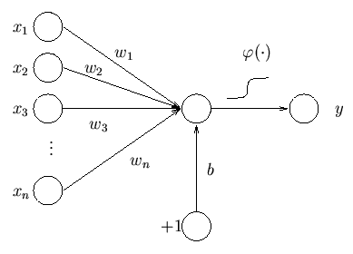
Here’s one where the weights use the variable “w” and the bias is explicitly shown as “b”. Here the sigmoid function uses the Greek letter “phi”, but more often you see the letter “sigma”.
A Little Math
So what do these diagrams mean about how we calculate the output from a set of inputs?
Notice first that we can have more than one output Y.
For K classes/labels, as in the digit recognition problem, we would have K outputs, and Y(k) = 1 if the label is the kth digit, otherwise it is 0.
The only exception is the 2-class case. In this situation, we only need 1 output because Y = 1 is the first class and Y = 0 is the second class.
We’ll focus on this scenario first.
The equation in its compact form is this:

The inside part is the dot product of the weights and the input:

As in linear regression we assume there is an x0 and that it is 1.
The “sigma” part is the sigmoid function:

If we graph the sigmoid, it looks like this:

There are 2 things we can tell from the above equation:
1) For logistic regression to work, the classes must be linearly separable. This is because the dot product between “w” and “x” is a line/plane.
(i.e. ax + by + c = 0)
w0 + w1x1 + w2x2 + … = 0 is the plane (more correctly, hyperplane) here.
So here is a situation where logistic regression would work well:

Here is a situation where it wouldn’t work well.

But we will cover that more in parts 2 and 3.
2) The sigmoid means the output Y is between 0 and 1.
So if w*x = 0, we land right on the hyperplane, and Y = 0.5.
If w*x > 0, we get Y > 0.5, and vice versa for w*x < 0.
As w*x approaches infinity, Y approaches 1, and vice versa.
Probabilistic Interpretation
Because Y is between 0 and 1, we can interpret it as a probability.
This makes more sense if you consider the following:
If we fall right on the barrier/plane between the two classes – our probability of being in either class is 0.5.
If we are further away from that barrier, the probability of being in either class increases.
We usually denote Y as P(Y=1|X) and P(Y=0|X).
Note that while we use some probabilistic concepts here, the way in which we use them is different than for say, a Bayesian classifier.
Also note that P(Y=0|X) = 1 – P(Y=1|X).
Maximizing the Likelihood
We have seen squared error used as an error function before, as with linear regression.
In fact, if we were doing regression, we could use the same thing here.
For classification, we take a different approach.
You may have seen this error function before:

t is the target and y is the output of the network/model. (This introduces some ambiguity because we usually write p(y=1 | x) as the output and y as the target).
This is called the cross-entropy error.
Where does this come from?
Let us go back to first principles.
Instead of minimizing error, we maximize likelihood. This seems like a logical place to start – maximizing the probability that our model parameters are correct.
Consider N IID (independent and identically distributed) training samples and corresponding labels (we’ll call them “t” here).
$$ L = \prod_{i=1}^{N} y_i ^{t_i} (1 – y_i)^{1 – t_i} $$
The likelihood of the model given the entire dataset can be represented by this equation. We can use the product rule because each sample is independent.
(Sidenote 1: This is the same thing we do when we want to say, find the maximum likelihood estimate for the mean. We calculate the joint probability aka. likelihood P(data|mean) and find the “argmax” mean that gives us the highest likelihood, hence the term – “maximum likelihood”)
(Sidenote 2: This is the same likelihood you see when we do Bayesian inference – posterior ~ likelihood x prior or P(param | data) ~ P(data | param) P(param))
(Sidenote 3: If you wanted to do regression, you would simply not have a sigmoid at the end, and you would use the squared error. The exponential of the squared error is a Gaussian, because in regression we often assume the error is Gaussian distributed. By making these 2 changes, we would just be doing linear regression.)
Recall y = P(y=1|x).
The target t can be 1 or 0.
When t is 1, only the left part of the product matters (the right side evaluates to 1). All the y’s here are the probability that the output of the network is 1. Given that the target is 1, we want to maximize this probability.
When t is 0, only the right part of the product matters. Recall that 1-y is the probability that the output of the network is 0. So when t = 0, we want to maximize this probability.
Since each sample is independent, we can get the joint probability by multiplying all the individual probabilities together.
2 key points:
1) There is no analytic solution, we must use iterative methods. In this tutorial we will cover gradient descent, but there are others (such as conjugate gradient, and L-BFGS).
The added advantage of learning gradient descent now is that it is also used to train neural networks.
2) As is usual with these ML problems, we will work with the log likelihood instead of the likelihood. Just try taking the derivative of both, and you will see why.
If you take the log of the above expression, notice you’ll get the same error function we started with!
We take the negative because we want something to minimize. We call this the “error” or “cost” function.
Maximizing the likelihood is equivalent to minimizing the negative likelihood.
It is also equivalent to minimizing the negative log-likelihood. This is because log() is a monotonically increasing function.
Gradient Descent
How do we actually minimize the negative log-likelihood if we can’t simply set the derivative = 0 and solve for the weights?
This is where gradient descent enters the picture.
Note that gradient descent is just a numerical method – it can be applied whenever you want to solve for the minima of a function, not just for machine learning.
Here is a picture of what we’re trying to do:

We start at some random weight, w = random().
Then we update the weight by going in the direction of the derivative of the error function (slope), which we have previously stated is the negative log-likelihood.
With squared error it is easy to see that the error function is quadratic, and so we are descending down a parabola in that case. The minimum is global.
With log-likelihood the extremum is also global.
It may help to plot the function E(y,t) = tlog(y) + (1-t)log(1-y) to see why.
The equation for updating the weights is:

Here j indexes the dimension, so j = 1…D.
t indexes the iteration number (not to be confused with the other t, which was the target).
“Eta” is called the “learning rate”. This hyperparameter determines how far along the error surface we travel on each iteration. Bigger values mean we go further, which means our weights might converge to the final solution faster, but it also means we may “overshoot” that solution.
Since w is a vector, we can usually speed up our code by doing vector operations (i.e. in MATLAB or Python). In this case, we can use this equation:

The full training algorithm is:
for i = 1…number of epochs:
error = negative log-likelihood ( -L(Y|X,w) )
w = w – learning rate * error gradient
The number of epochs is yet another hyperparameter. There are many ways to determine when to stop the gradient descent process.
Some other methods you may want to look into:
- Stopping when the gradient is small enough
- Stopping when the training error is no longer decreasing or approaching 0
- Stopping when the error on a held out test set starts to increase (overfitting)
We call things like learning rate and epochs “hyperparameters”. These are parameters that are not part of the model itself, but can still be optimized, perhaps via cross-validation.
Biological Inspiration
In computational neuroscience, a logistic regression unit is sometimes referred to as a “neuron”. How are the two related?
Here is a diagram of a typical neuron.

Some notable components:
- Dendrites: These are the “inputs” into the neuron – they take electrical signals from other neurons’ axons.
- Cell body / Nucleus: This part of the neuron “sums up” all the inputs and propagates this summed signal to the axon.
- Axon: This is the “output” of the neuron. It sends the signal from this neuron to other neurons’ dendrites.
So dendrites are our logistic unit’s X, and axons are the Y.
The brain is essentially a network of neurons, or rather, a neural network. An artificial neuron network, which is the topic discussed in Part 2 of this tutorial, is a network of connected logistic regression units.
Another notable feature of neurons is the behavior of the “action potential”.
Observe a typical amplitude/potential (voltage) vs. time signal:

Notice how the potential rises gradually and then spikes. We call this the “all-or-nothing” principle. If the sum of the inputs to the neuron is high enough, a spike is generated. Otherwise, the voltage stays relatively low.
This is reflected in the logistic units’ binary output. The output if a sigmoid is interpreted as P(Y=1|X) – the probability of being “on”, or in other words, the probability that a spike is generated.
Inhibitory vs. Excitatory neurons:
It is well-known that the signal a neuron sends can either “excite” or “inhibit” the receiving neuron. These are reflected in the logistic model by the weights. A positive weight is excitatory. A negative weight is inhibitory.
Researchers have tried to create models with “spiking” neurons, however, it has been difficult to get them to actually learn anything.
Where can I learn more?
The topic of this post (logistic regression) is covered in-depth in my online course, Deep Learning Prerequisites: Logistic Regression in Python. We derive all the equations step-by-step, and fully implement all the code in Python and Numpy. To solidify the concepts, we apply the method to real world datasets, including an e-commerce dataset and facial expression recognition.


