
Deep Learning Tutorial part 2/3: Artificial Neural Networks
Lazy Programmer
This is part 2/3 of a series on deep learning and deep belief networks.
This section will focus on artificial neural networks (ANNs) by building upon the logistic regression model we learned about last time. It’ll be a little shorter because we already built the foundation for some very important topics in part 1 – namely the objective / error function and gradient descent.
We will focus on 2 main functions of ANNs – the forward pass (prediction) and backpropagation (learning). Your sci-kit learn analogues would be model.predict() and model.fit().
As with logistic regression, we have some set of training samples, X1, …, Xn, and we will use gradient descent to learn the weights of our model. We then test our model by computing predicted outputs given some test inputs (the forward pass) and comparing them to the true outputs.
This topic is covered in-depth in my course, Data Science: Deep Learning in Python. We derive all the equations by hand, step-by-step, and we implement everything using Numpy and Python. To solidify the concepts, we apply the method to some real-world problems, including an e-commerce dataset and facial expression recognition.
Prediction
As with logistic regression, we will start with a diagram / schematic of a neural network.
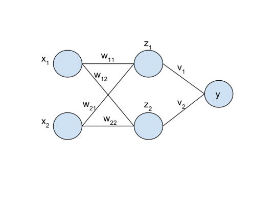
We call the column of x’s the “input layer”, the column of z’s the “hidden layer”, and the column of y’s the “output layer”.
As in part 1, we will only use one y (binary classification) for most of the tutorial. Recall that the only difference is that when you have more than one output, you use the “softmax” output function. The methods (calculating the gradients for gradient descent) remain the same.
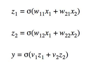
Each of the variables can be computed as follows:
z1 = sigma( x1*w(1,1) + x2*w(2,1) )
z2 = sigma( x1*w(1,2) + x2*w(2,2) )
y = sigma( z1*v(1) + z2*v(2) )
We can combine each of the weights w(i,j) into a matrix W – this is useful for coding in languages like Python and MATLAB where matrix and vector operations are much faster than for-loops. The size of W will be N x M where N is the number of x’s and M is the number of z’s.
Similarly, v(j) can be combined into a vector V of size M.
If we had more than one output for y, V would be a matrix of size M x P, where P is the number of y’s.
As in part 1, “sigma” refers to the sigmoid function, but other functions may be used. The hyperbolic tangent, or “tanh” is sometimes used – it is just a vertically scaled version of the sigmoid. Both make it relatively easy to compute the derivatives for gradient descent later on.
If you look at how we compute z1, z2, and y closely – you’ll recognize that these are all just the logistic regression formula. In fact, an artificial neural network is just a combination of multiple logistic regression units put together.
This is the neural network with one logistic unit highlighted:
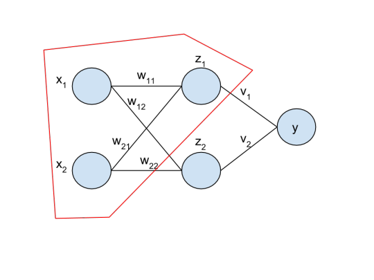
One way we interpret this is that z1 is some “feature” extracted from (x1,x2), weighted by (w(1,1),w(1,2)), and similarly for z2.
Then y is a logistic regression on (z1,z2) – the features learned from the input.
This all begs the question – why use neural networks in the first place if we are just going to add a bunch of parameters and make it look more complicated?
Recall that logistic regression only worked on linearly separable problems. For example, you couldn’t train a logistic regression unit to learn the XOR function because you can’t draw a line between the classes.
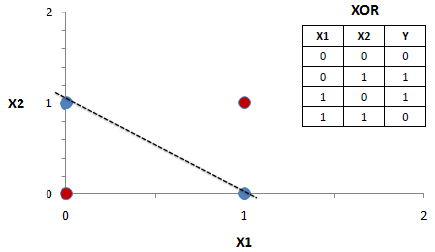
What you could do if you really wanted to use logistic regression, is create another input x3 = x1*x2. As an exercise, convince yourself that this works. Hint: try [w0,w1,w2,w3] = [-0.5,1,1,-2].
The problem with the above approach is that you had to come up with the extra feature (x3) manually. You don’t know ahead of time what will work and what won’t. Real machine learning problems can have hundreds or thousands of inputs – you can’t try every combination possible. We haven’t even considered other functions. What about sin(x)? x^2 or x^3? log(x)? There are infinitely many features we could extract.
The beauty of neural networks is that they learn these features automatically. As an exercise, try manually assigning weights to a neural network with 3 hidden units that can compute the XOR function at y.
Another way of stating what we have just learned – artificial neural networks can learn nonlinear functions.
Learning aka. Backpropagation
Learning the weights for a neural network is very similar to logistic regression. We will follow the same method here – write out the objective function we want to minimize, calculate its derivative with respect to the parameter we want to update, and use the gradient descent algorithm to perform the weight update.
In fact, the steps remain the same:
for i = 1…number of epochs:
    error = negative log-likelihood aka. -L(Y|X,W,V)
    w = w - learning rate * error gradient wrt w
    v = v - learning rate * error gradient wrt v
The only difference now is that the likelihood depends on W (which was 1-D for logistic regression and is now 2-D) and V – since Y depends on W and V.
Even the objective function J remains the same as with logistic regression – it only depends on the output y and the target t – and will be the squared error or cross-entropy depending on the problem.
Calculating the gradient for any v(j) is simple because y depends directly on V and by the chain rule:
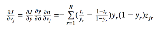
Here we’ve assumed we’re using the cross-entropy error, R is the total number of training samples and we index them by r – running out of letters!
The gradient for W is a little more complicated because it involves calculating the “total derivative”. If you have more than one output y(k), k=1…P – then the objective function will depend on all the y’s. At the same time, each y(k) will depend on the same w(i,j).
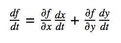
In general, if you have a function f(x,y) where x(t) is a function of t and y(t) is a function of t, you can write the “total derivative” of f(x,y) as:
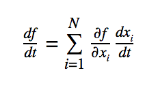
For a vector x with N components, the above can be generalized to:
If we replace f() with the objective function J(), t with the weight w(i,j), and each component x(i) with the outputs of the neural network y(k), k = 1…P, we get the following:
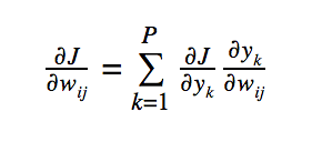
Note that we can expand the right-most derivative so that we take the derivative of y(k) with respect to z(j), multiplied by the derivative of z(j) with respect to w(i,j). The latter term does not depend on k, so it can be removed from the summation.
Although this may seem now like a straightforward application of vector calculus – don’t be fooled – it took researchers many years to figure out how to solve this problem. Read more on Wikipedia.
Multi-layer neural networks
So far we have looked at neural networks with only one hidden layer, but neural networks can have any number of hidden layers, with any number of dimensions per layer. (You will need to apply the total derivative rule recursively for each layer going backward).
You may want to do your own research as to what type of architectures will work best for your problem.
Neural networks almost give us too many choices – how many layers should I have? 1? 3? 100? How many units per layer? 500? 10000? 10001?
Of course, adding layers and units will only increase the time in takes to train your neural network. Every layer you add will result in an increase of N1 x N2 parameters to your model – where N1 is the number of inputs into the layer and N2 is the number of units in the layer that receives the inputs.
Thus neural networks can be very prone to overfitting. Suppose we are training a network with one hidden layer, where the input is a 32 x 32 image, the hidden layer has 500 units (i.e. 500 features extracted), and the output is 10 (because the images are handwritten digits from 0 to 9).
That’s 32 x 32 x 500 parameters for W, and 500 x 10 parameters for V. That’s 517 000 parameters!
One “rule of thumb” I’ve seen is that you want the number of training samples to be at least 10x the number of parameters. So for the example above, you’d want at least approximately 5.2 million samples to train from.
So you don’t want to needlessly add more layers and more units to your neural network just to make it more expressive.
One well-known result from neural network literature is that neural networks with as few as one hidden layer are “universal approximators” (i.e. they can approximate any function). Source: http://www.sciencedirect.com/science/article/pii/0893608089900208
Where can I learn more?
This topic is covered in-depth in my course, Data Science: Deep Learning in Python. We derive all the equations by hand, step-by-step, and we implement everything using Numpy and Python. To solidify the concepts, we apply the method to some real-world problems, including an e-commerce dataset and facial expression recognition.


